9.5. RADIOMETRIC TRANSFORMATIONS AND IMAGE ENHANCEMENTS

Various methods have been developed for the analysis of multi-channel satellite data using their multispectral nature for radiometric transformations and image enhancement. These techniques play a fundamental role in image interpretation. Most methods may either be applied to uncalibrated data sets or to preprocessed image data sets.

9.5.1 Image ratios

Image ratios are the basis of a simple algebraic method used for feature extraction, reduction of terrain illumination effects, image enhancement, computation of vegetation indices and more (this topic is widely discussed in various papers, for example, refer to Mather, 1999:117-124). To understand a particular channel ratio formula, the object reflectance curves have to be considered (sample curves for green vegetation, soil and water are shown in Figure 9.2). In general, the ratio result for pixels with very different values for the input channels is larger (brighter) than for pixels with similar values. The image ratio equations can be computed with r.mapcalc. It is important to include a multiplier of 1.0 at the beginning of the map algebra expression because we are dividing integer values. Otherwise, the result will become zero and not the expected floating point numbers. As an example, we calculate a ratio between LANDSAT-TM5/7 channel 7 and 4:

r.mapcalc ratio7.4=1.0 * tm.7 / tm.4

For more than 15 years, a variety of vegetation indices have been developed. To illustrate such a calculation, we can compute a NDVI map (normalized difference vegetation index) from LANDSAT-TM5/7:

r.mapcalc ndvi=1.0 * (tm.4 - tm.3) / (tm.4 + tm.3)

For the calculation of NDVI, the differences between the red and the infrared channel are taken into account pixel-wise to derive information about the vegetation cover. When a pixel value in the near-infrared dominates over the red wavelength (as for green, healthy vegetation), the NDVI is positive. NDVI for unvegetated soil will be slightly above zero; for water, below zero. To quickly classify these three (or more) landcovers, you may filter them with r.mapcalc (if-condition).

9.5.2 Principal Component Transformation ( 1

Multispectral image channels often contain correlations due to similarities of the spectral response of the observed objects or slightly overlapping filter

functions of the spectral sensors. This leads to redundancies within the data set. The Principal Component Transformation (PCT) method has been developed to transform such a data set to a new data set without correlations between the channels. This will concentrate the image information in fewer image channels (reduction of image dimensionality), which is of particular interest for hyperspectral data. The PCT transforms the original multispectral data set to a new spectral coordinate system, the Principal Component axes, which are orthogonal to each other. Figure 9.10 shows the position of original multispectral pixels and the PCT coordinate system. In general, the first principal component (PC) image contains the maximum possible variance of the original images. The second principal component image contains the maximum possible variance not stored in the first PC image, as the second PC axis is orthogonal to the first PC axis (Schowengerdt, 1997:191). Accordingly, higher PC images explain remaining variances. The number of PC images is identical to the number of input channels. Since the amount of variance decreases from the first to the last PC, uncorrelated noise (and sometimes some remaining high frequencies) is found in the last PC image. As a results, the method is sometimes used for image compression, as it allows the image information to be concentrated in fewer channels. PCT is also sometimes used to generate additional channels to obtain more variables for a later reclassification process.

The scatterplot in Figure 9.11 shows the original spectral axes and, after transformation, the new rotated PC axes for a sample LANDSAT-TM5 pixel cloud (channel 3 and 4).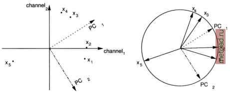

Figure 9.10. Left: Multispectral pixel values shown as standardized data vectors ito jc; with related first and second orthogonal principal component vectors PCT1 and PCT2 in coordinates view. Right: Same data vectors in circle coordinates view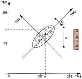

Figure 9.11. Principal Component Transformation applied to channels tm3 and tm4 of a LANDSAT-TM5 data set. Both the original spectral axes (channels tm3, tm4) and the PC axes (PCT transformed channels tm3, tm4) are shown

In GRASS, the Principal Component Transformation is implemented in i.pca. The module requires the input channel names (at least two images) and a prefix for the transformed PC image files, which will be enumerated incrementally. Optionally the data can be rescaled to a range different from the default range of 0 - 255.

Another method not covered here is the Fourier transformation, which is provided by i.fft and i.ifft (forward and backward transformation). It transforms image data from spatial to frequency domain. Among the important applications of the Fourier Transformation are the identification and elimination of (periodic) noise or stripes in a satellite image.

9.6. GEOMETRIC FEATURE ANALYSIS

The geometric (spatial) feature analysis applies local neighborhood operations to raster data. Several methods are available for image smoothing: contrast improvement, low- and high pass filtering, edge detection and more. Geometric filters are user defined raster matrix templates ( moving window ) moving row- and column-wise over the image used to calculate the new raster map. All raster cells which are covered by this moving window are considered for the calculations.