vector intersection the existing lines have to be broken and a new node has to be inserted (compare Figure 6.4). Please note that in GRASS 5.3, all vector modification tools ignore the current geographic region settings and always operate on the full map. The map boundaries are extracted from the vector file headers. As an example, we patch the soils map with the farm fields map (Spearfish region):

V.patch in=soils,fields out=soilsfarms.patch v.info soilsfarms.patch

In the resulting intersection map soilsfarms.patch, the boundaries of the geographic region will be expanded to encompass the maximum geographic region as defined by the patched maps. The scale will be set equal to the smallest (i.e., most gross) scale used by any of the patched map layers. Remember that the scale will affect the node-snapping thresholds as implemented in v.digit, v.support and v.spag. The v.info command confirms that no topology is present yet. This has to be built with v.support:

v.spag -s soilsfarms.patch v.support soilsfarms.patch

As there is no duplicate line removal in v.patch, the new map has to either be edited with v.digit or cleaned with v.spag. The latter must be done with care as explained above.

Clipping vector maps. To clip a vector map to modified map boundaries the script v.cutregion.sh is available. You first need to change your current region to the region of interest with g.region or d.zoom. Then you apply the script v.cutregion.sh which clips the vector map according to the current region settings and writes a new vector map.

A vector map intersecting tool which takes into account the shape of polygons is v.cutter. This module generates a new map based on an intersection of two input maps, cutter and data. The map cutter determines the active areas for the input map while data delivers the area contents. The attributes of created polygons will be generated from the attributes of the data map. As an example, we cut out the soils only for areas present in the map rstrct.areas: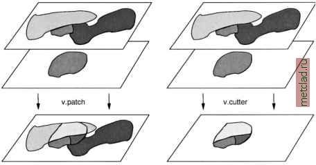

Figure 6.5. Possible results of intersecting vector data using v.patch or v.cutter

The new map contains soil information only for the restricted areas. This is also a convenient way to create masks based on vector maps.

To mask vector maps based on this method, you may digitize a mask area with v.digit or generate it with other tools. The mask area should be labeled with a category number (e.g. 1). The vector areas will determine the outline of the final vector map. The module v.cutter produces a new map that contains all the vector data from the data map that fall into the extent of the vector mask map given as map cutter. Figure 6.5 illustrates the difference between v.patch and v.cutter.

6.3.3 Map reclassication

Vector maps can be reclassed in a similar way as raster maps. The module v.reclass reclassifies vectors according to user defined reclass rules. The module is used in a similar way as r.reclass. As an example, we can reclass the fields map into two categories: private and Black Hills National Forest . The ASCII table containing the reclass rules can be written with any text editor. It will contain:

1 thru 62 = 1 private

63 =2 Black Hills Natl. Forest

This table will be applied to the map to generate a new reclassified vector map. The module v.report can then be used to get the list of input categories:

v.report fields type=area

cat fields.reel I v.reclass fields type=area out=fields.reel

The new map contains only two categories. With flag -d you can dissolve common boundaries of adjacent polygons with same category assigned during the reclassification. Note that there are parallel lines in the Spearfish fields map which represent roads.

6.3.4 Feature extraction from vector data

To extract vector objects from a vector map, you can run v.extract with the desired category(ies) listed by the parameter list. This will extract the selected vectors into a new map. As an example, we can extract the fields owned by C. Mitchell into a new vector map. We can get the category numbers of the vector polygons from v.report:

v.report fields tYpe=area

v.extract fields type=area out=fields.mitchell new=0 list=10-15 d.vect.area -r fields.mitchell

The parameter new is set to zero to keep original categories, optionally, a new category number can be specified. For a larger list, the selection can be written into a file, and its name is then specified as the parameter file. The new vector map contains only the selected areas. You can dissolve common boundaries when adjacent polygons have the same category by using the command with the flag -d.

6.4. VECTOR DATA TRANSFORMATIONS TO/FROM RASTER AND SITES

First, we explain the transformation of raster and site data to the vector data model, then we show how to change vector data to rasters. Depending on the type of geographic phenomenon that the vector data represent, we distinguish two types of transformation from vector data to raster:

for geometric features (points, lines, areas) we use direct transformation from vectors to raster lines/areas or sites;

for continuous fields (isolines, contours) we need spatial interpolation to transform from vector lines to rasters;

feature extraction from raster objects to vectors requires vectorization. Figure 6.6 shows an overview of available conversion techniques.